DAX is a language of sub-formulas; what at first looks like one big formula is usually several sub-formulas chained together. We talked about this last time, and I hope the idea is starting to make sense in your head, even if slowly.

And like we talked about last time, the two main types of sub-formulas you need to understand are “Per Row Formulas” and “New Filters Formulas”. The former being used within Iterators (argument 2) to describe what you would like to do for each row of a Temp Table, and the latter being used within the CALCULATE function (argument 1) to describe what you would like to do after changing the filters in some way.

Now, when DAX is running *any* of these sub-formulas, in order for that sub-formula to produce the desired answer, it could potentially need to have access to two different pieces of information:

(1) What row the sub-formula is running in. (If it’s running in a row.)
(2) What filters are in place when the sub-formula runs. (If there are any.)

To handle this, DAX keeps track of this information in two dedicated lists*:

Row Context is the list of all the values in the current row.
Filter Context is the list of all the current filters.

Every time a sub-formula runs it will *always* have a pair of these lists set up for it (even if one or both of the lists are empty). This way, if the sub-formula needs to know about “what’s in the current row” or “what filters are in place”, it can pull that information from one of the two lists.

Rephrased slightly: every time a sub-formula runs, DAX always provides that sub-formula with both a list of all the values of the current row (Row Context) and a list of all the current filters (Filter Context).

If there are no values of the current row (because the sub-formula isn’t running within a row), then the first list (Row Context) will be empty; if there are no filters currently in place, then the second list (Filter Context) will be empty. Both lists can be empty, but in that scenario the sub-formula is still handed two empty lists so it can see that there are no values in the current row and there are no filters currently in place.

This combination of “one Row Context and one Filter Context” that have been set up for a given sub-formula is called the Evaluation Context of the sub-formula. So “Evaluation Context” is simply a pair of lists that provides important information to a sub-formula about what’s in the current row, and what filters are in place. When we say “The sub-formula runs within an Evaluation Context”, we simply mean that it runs using the specific pair of lists that were set up for it.

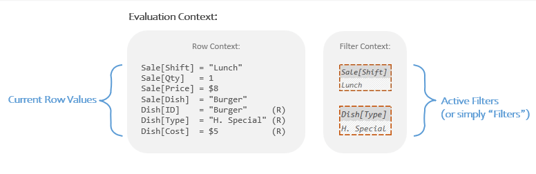
Before we go any further, here’s a sample illustration of an Evaluation Context which might make the ideas a little more concrete:

On the left we can see the Row Context and on the right was can see the Filter Context.

Our fancy name for each item in the Row Context is a Current Row Value, which is simply a value from one of the columns in the current row (the little “(R)”s indicating that the column is a Related column). Our fancy name for each item in the Filter Context is an Active Filter, which almost always is shortened to just “filter”.

OK, that’s all well and good; but what does the sub-formula actually do with these lists? What jobs do the lists actually perform?

The job of the first list (“Row Context”) is to simply store all the values of the current row so that the sub-formula can easily grab them and use them. Rephrased: Row Context is *where* a sub-formula goes to grab values from the current row. Usually this is as simple as typing the name of the column that has the value you want (“Sale[Qty]” or “Sale[Price]”) but it can also involve specialty functions like RELATED, EARLIER, or EARLIEST if the desired column is a Related column (it has a little “(R)”) or if there are multiple columns sharing the same name (much less common).

The job of the second list (“Filter Context”) is to store all the filters that need to be applied automatically if the sub-formula contains a function or reference that involves an Auto Filtering step. The Auto Snapshot is the example of this that we’ve talked about most, but several very common functions like SUM, MIN, MAX, and AVERAGE all include an Auto Filtering step, which is why (or more accurately *how*) those functions respond to slicers automatically.

Let me show you that same image again so you don’t have to scroll back up:

If you were to ask a sub-formula about this Evaluation Context it would say:
“Looking at the Row Context I can see the current row has values from 7 columns I can grab; and looking at the Filter Context I can see there are two filters that need to be applied if I do anything that involves Auto Filtering.”

This concept of Evaluation Context is both easy and tricky at the same time. This is because the concepts of “the current row” and “the current filters” are fairly intuitive and it seems odd to complicate things by imagining them as lists. What’s easy to forget here though, is that the thing running all of our DAX formulas is a computer, and that computer needs a computer-friendly way to keep track of both of these pieces of information. That’s all Evaluation Context is, a computer-friendly way of keeping track of what’s in the current row, and what filters are in place.

In the next two articles we are going to dive into these concepts using examples from the previous posts. By the end you should understand how all of this works a whole lot better.

*A couple notes just for the very technical folks:

I use the term “list” here, a more appropriate term might be “collection”. I’ve found though that “list” conveys the exact right *idea* for most people and is much less intimidating than “collection”. When reading ahead, feel free to swap out any instance of “list” with “collection” if that works better for you.

Also of note, what really gets stored in these lists are more like *pointers* to the values of the current row and *pointers* to all active filters. So when we say the Evaluation Context provides information about the values in the current row and the active filters, we can be more specific and say Evaluation Context is providing a way for a sub-formula to both easily go grab any value of the current row and easily go grab all the active filters.

Lastly, as I’ve mentioned in previous posts, what I call “formulas” and “sub-formulas” are called “expressions” and “sub-expressions” elsewhere. The latter terms are more technically accurate, but the former I find much more accessible and less intimidating to new users. Again, they convey the correct *idea*, which I believe is more helpful for new folks.

Setting Things Up

If you’ve been following along, you’re probably very used to my Data Model for the not-very-busy restaurant with a rather dull menu. If you’re not though (of if you just love seeing it over and over) here’s it is again:

We have a “Sale” table, a “Dish” table, and a relationships between them from “Sale[Dish]” to “Dish[ID]”.

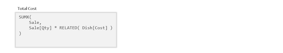
Today we’ll be using our “Total Cost” Measure that we’ve used several times before:

Total Cost =
SUMX(
    Sale,
    Sale[Qty] * RELATED( Dish[Cost] )
)

In this simple Measure we start with the SUMX function. SUMX wants a Temp Table (argument 1) and a Per Row Formula (argument 2).

The Temp Table we’re giving SUMX is the Auto Snapshot of “Sale”. (More info here)
The Per Row Formula is on line 3.

Here’s that Per Row Formula pulled out so we can look at it in isolation:

Sale[Qty] * RELATED( Dish[Cost] )
 

That is the sub-formula that will run once per row of the Temp Table. Our next step is to dive deeper into how DAX actually does that.

Mechanically DAX is going to create a pair of lists for each row (one Row Context and one Filter Context) and then run the sub-formula within each pair of lists.

If that paragraph probably gave you a headache, that’s OK. It’s not that different from what you’ve already learned, it’s just more mechanical.

Images will help here.

Regaining Our (De)composure

Let’s imagine our Measure running in a Power BI card visual:

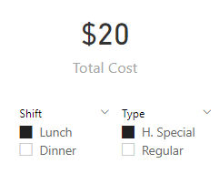
Note that the user has sliced down to both “Lunch” and “H. Special”. That will become important in a minute.

Our main question though, is where did that “$20” come from? Or more specifically, what role did Evaluation Context play in coming up with that “$20”?

To begin answering, let’s simply imagine our Measure in a little box…

…and the first big thing we’ll do is “decompose” it. To do this, we’ll visually pull the Per Row Formula (a “sub-formula”) out into its own box in its own “panel”. Eventually each panel will show us how formulas/sub-formulas interact with different Evaluation Contexts. We’re getting ahead of ourselves though, right now lets just pull the sub-formula out:

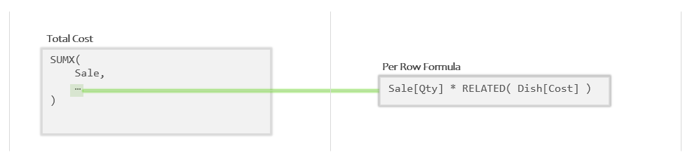
So we see the main formula for the Measure in the left panel and the Per Row Formula broken out in the right panel.

(Rephrased: the left panel holds the “parent formula” and the right holds the “sub-formula”)

Remember those slicers the user clicked on? Let’s incorporate those into our illustration by adding the Measure’s initial Evaluation Context. We’ll add it at the bottom of the *left* panel because it’s just the stuff in the left panel that uses it (the right panel will get its own Evaluation Contexts momentarily):

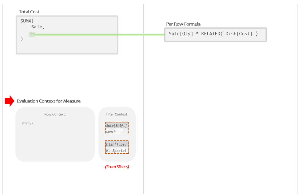
That is the initial Evaluation Context the Measure starts running within. The Row Context is empty because, well, we’re not “in a row” yet; and the Filter Context has two filters from the slicers on the Power BI page.

So as far as the formula in the top left box is concerned, there are *zero* values of the current row that can be grabbed (Row Context is empty), and there are *two* filters that will be applied during anything that performs Auto Filtering (Filter Context has two Active Filters).

Speaking of which, if you’ll remember, argument 1 of SUMX is the Auto Snapshot of “Sale”. All Auto Snapshots perform Auto Filtering, so the Temp Table that comes out is going to be affected by the two filters in the current Filter Context. Let’s see what that Auto Snapshot produces:

The Auto Snapshot of “Sale” made a copy of the “Sale” table, added Related Columns, and then performed Auto Filtering . During Auto Filtering, it was those two filters in the left panel’s Filter Context (“Lunch” and “H. Special”) that got applied. The resulting Temp Table has two rows (the “Lunch” and “H. Special” ones) and you can see what it looks like in the blue bubble just above the box.

(If you need to “zoom in” on the above image, feel free to right click on it and open it in a new tab)

OK, so next, SUMX wants to run the Per Row Formula once per row of *that* Temp Table.

Here’s where things get interesting.

Because our Temp Table has *two* rows, SUMX creates *two* new Evaluation Contexts. They are based on the Evaluation Context in the left panel, but each has the information of a different row of that Temp Table written down in the Row Context list. These Evaluation Contexts are what SUMX “slips underneath the wall” between the two panels to give to the Per Row Formula:

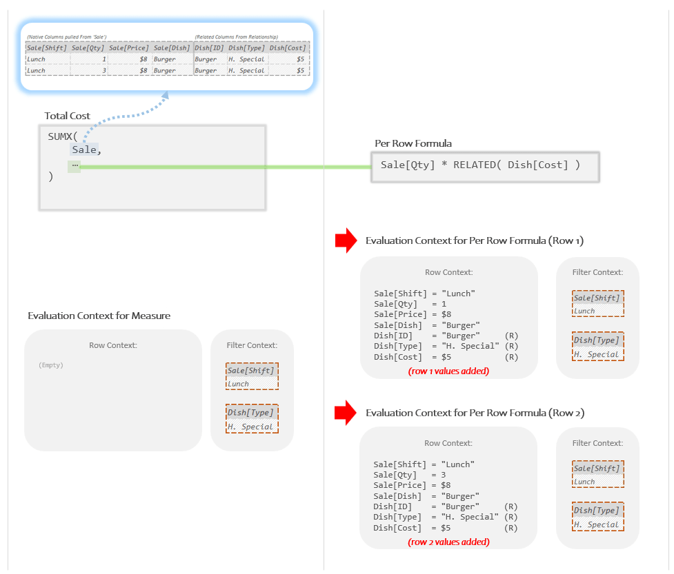
So each row of the Temp Table in the top left is represented as a new Evaluation Context in the bottom right. Look close and you’ll see that all the values of each row have been written out into the two new Row Contexts.

It’s worth noting that the Per Row Formula can’t “see” into the left panel where the Temp Table is (the wall separating the panels is “in the way”), however it can see the two new Evaluation Contexts that SUMX “slipped underneath the wall”. Evaluation Contexts in this light can be understood as the tool that parent formulas use to communicate important information to their sub-formulas.

OK, that’s more than enough theory; back to the task at hand.

With the two new Evaluation Contexts set up, the Per Row Formula can be run twice, once within the Evaluation Context for row 1, and a second time within the Evaluation Context for row 2. Let’s see what that looks like:

In the Per Row Formula, the references of “Sale[Qty]” and “RELATED( Dish[Cost] )” both tell DAX to go looking for a number in the current Row Context with the equivalent column names. (The RELATED function indicating that the value is from a Related column and hence will have a little “(R)” next to it.)

When running in the Evaluation Context for Row 1, when DAX goes looking in the Row Context it grabs the numbers “1” and “$5” (highlighted in yellow).

When running in the Evaluation Context for row 2 it grabs the numbers “3” and “$5” (highlighted in purple). Because this Row Context is storing values from row 2, the same references result in different values being grabbed.

Both times we can see that Row Context really is just a place where the sub-formula goes to *grab* values; essentially by name. Our sub-formula has the names of the columns we want and the Row Context is where the values associate with those columns are stored. (The RELATED function adds a little complexity around grabbing values from Related columns, but just a little). Keeping track of all this in your head takes practice, but conceptually it’s pretty simple: Row Context is where the sub-formula goes to grab values of the current row.

OK, after grabbing the pair of numbers for each row, the pairs are multiplied together, just like the Per Row Formula asked. This gets us “$5” for the first row (1 * $5) and “$15” for the second row (3 * $5). Those are the numbers that get summed up to come to our final answer of “$20” we saw in Power BI:

That’s how DAX uses Evaluation Contexts to run the Per Row Formula “once per row”. It’s almost more like “once per row’s Evaluation Context”. All of this is not that different that what we’ve talked about before, it’s just more mechanical.

(BTW our fancy name for these references in the Per Row Formula are Current Row References. A “Current Row Reference” is anything that goes and grabs a value from the Row Context. The most common example is when you just type in the name of the column like “Sale[Qty]”. Next most common is wrapping a column name in the RELATED function to indicate the value you want in the Row Context is from a Related column and hence has a little “(R)” next to it (“RELATED( Dish[Cost] )”). There are also less common versions that use the EARLIER and EARLIEST functions that handle situations where the Row Context has two values with the same column name; an unusual occurrence and a topic for a future post. For now don’t worry too much about the fancy names.)

A Literary View

So a couple posts back, we were working through the exact same Measure and I had an image showing the Per Row Formula being run for just the top row of our Temp Table:

This image was both much simpler and much easier to understand than what I went through in the last section. The above image is also how I see things day to day. It’s a very useful and good way to understand things.

As you might be thinking though (since I’m bringing it up), it is technically a little bit off. Just a little bit though. Armed with our new found knowledge of Evaluation Context I can make the above image more accurate with just two small changes:

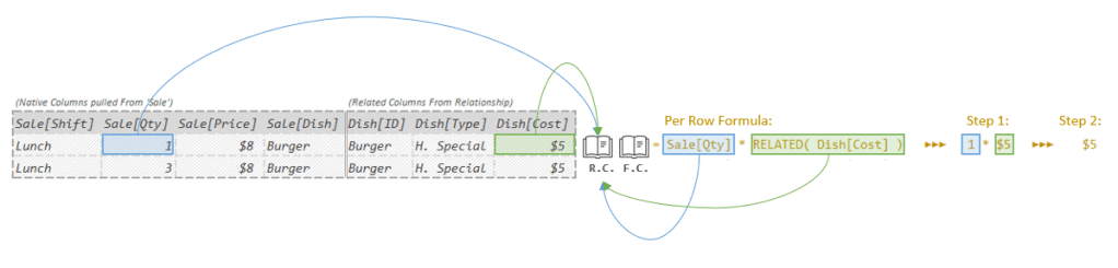
Notice the two books in between the Temp Table and the Per Row Formula? Those are the Row Context (R.C.) and Filter Context (F.C.) for that top row.

When SUMX creates an Evaluation Context for each row, you can just imagine those Evaluation Contexts as two little books where the “list of values of the current row” and “list of active filters” for each row are stored for the Per Row Formula to use.

Then when the Per Row Formula needs to grab values for the current row, it just goes and “looks in the book” where that information is kept. Said otherwise, it looks in the Row Context.

So, to be extra clear, when the Per Row Formula runs, it doesn’t actually look directly into the Temp Table to find the numbers for the current row, it looks in the Row Context where those numbers have essentially been “staged” for it. That’s the main reason that list exists. Or if you prefer, Row Context is the thing whose job is to provide visibility into the current row.

(To use slightly fancier terminology, the Row Context is the thing that *exposes* the values of the current row to the sub-formula).

Time for a Pastry Break

Initially I wanted this to be a single post, but I think at this point you should probably take a break to digest what we’ve just gone through. Go find yourself a little treat, you’ve earned it.

When we return we will talk more on Filter Context and how you can use CALCULATE to change it. That should be a shorter and easier post.

Till next time!

-BG

Post Script: More Detail Than You Want to Know

This last bits just for the technical folks or the folks with a lot of DAX already under their belt. Other folks should skip this.

OK, when I started I showed you this image:

Which says the Row Context is a list (or “collection”) or Current Row Values.

In practice, this is how I describe things; but if we want, we can be a bit more specific. Here’s a more nuanced dissection of a Row Context as I understand it:

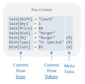
The Current Row Values are actually just the numbers and text strings (the “scalar values”). The column names we can call the Current Row Keys, which are essentially the names or “lookup keys” for the values. The last bit in parathesis we just call meta data. (There’s a few more pieces of meta data I haven’t shown you yet, but it’s all just meta data.)

Therefore each “thing” in the Row Context can be well understood as a pairing of a key, a value, and some meta data.

So when we say:
“Row Context is a list of Current Row Values”

We could be a bit more accurate and say:
“Row Context is a list of Current Row Key-Value pairs with associated meta data.”

But that doesn’t exactly roll off the tongue, does it? Despite potentially being more accurate this second version has unnecessary detail for new folks and frankly old folks as well. The simpler version is I think much better.

This use of a Key-Value Pair concept may be very familiar to you but should not necessarily be taken literally. What I’m trying to give to you is a way to model Row Context in your head that is simultaneously easy-to-understand and very reliable. I don’t know how this is implemented internally in DAX but I know I rely on this mental model daily and to the best of my knowledge it has yet to fail me once. It’s made working with DAX much, much easier for me.

(Lastly, for those wanting to email me about how USERELATIONSHIP or EARLIER fit into things; don’t worry, that’s coming, it’s just a few more posts off.)