In the last post we looked at how if you can properly understand and visualize the Auto Snapshot, understanding the RELATED function is actually quite simple.

The Temp Table produced by the Auto Snapshot has several columns added during the Super Lookup (aka “Table Expansion”). These added columns are classified as Related columns. While these columns are primarily added to support Auto Filtering they can be used for other things too.

If you pass the Temp Table into an Iterator like SUMX, in your Per Row Formula you can get at the value of any of these Related columns in each current row simply by using the RELATED function paired with the name of whichever column you want to use.

I really like how much this simplifies the inner workings of RELATED. Maybe more importantly, when you go to write your Per Row Formulas, instead of thinking of several Model Tables with relationships between them, you can imagine just one single very wide Temp Table, with all the columns you need.

Another place where understanding and properly visualizing the Auto Snapshot can come in handy is with any of the grouping functions. The two main grouping functions are SUMMARIZE and GROUPBY.

In this post we will look at GROUPBY, and how when paired with the right imagine in your head it can elegantly solve what otherwise might feel like an impossible problem with just few lines of code.

Before we can go further though, we have to switch to a different Data Model though.

So goodbye “Burger, Pasta, and Salad”, hello “Donuts and Hot Cocoa”.

A Good Start: Donuts and Hot Cocoa

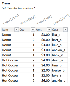
In this new Data Model we actually have fairly similar data; it’s still about food sales (retail sale data makes for easy to follow demos), but this time we can imagine it’s a little donut stand that just sells donuts and hot cocoa.

We have a “Trans” table that has all of our sales transactions and a “Cust” table that lists out all of our customers:

The question we are interested in is:

“How many Households (not individual customers) have we sold to?”

Let’s take the above image and add an example visual with slicers to the right:

If we notice the users has sliced to look at Donut sales, which means we are looking only at the first five rows in the “Trans” table on the left. The Measure is returning 3. Do we trust it? Well, a smart human can look at the tables and note that:

Lisa and Bart Simpson’s purchases (row 1 and 2) count as one household,
Luke and Anakin Skywalker’s purchases (row 3 and 4) count as a second household,
Hank Venture by himself (row 5) counts as a third household.

So our Measure is returning the right answer; we sold donuts to 3 households.

So that’s how a human could figure out the answer. But how do we get DAX to do what seems so simple for humans?

Easy, Peazy, Lemon Squeezy

I’ve seen many many approaches to this kinda of problem that span 30 or 40 lines of dense code. Here’s mine:

Households Sold To =
COUNTROWS(
    GROUPBY( Trans, Cust[Household] )
)

That’s it. Three lines.

How does it work though?

COUNTROWS we’ve seen before and is easy to understand, what about GROUPBY though?

The good news is that GROUPBY’s basic use isn’t too tricky.

If you’ve got a Temp Table, and you want to keep just the unique combinations of a couple of its columns, or you just want the unique values of just one single column; GROUPBY is your friend. (It’s very much like “Remove Duplicates” in Excel)

Here’s the stuff that GROUPBY wants as a arguments:

GROUPBY( 
    <Temp Table>, 
    <Temp Column #1>,
    <Temp Column #2>,
    <Temp Column #…>
)

So argument 1 is always a Temp Table. All the arguments after that are just names of columns in *that* Temp Table you’d like to keep the unique combinations of. You can type in 1 column or as many columns as you’d like to keep the unique combinations of.

(I’m leaving off some other GROUPBY features here to stay focused on essential behavior. Also, you can also do this same thing with the SUMMARIZE function, but its name is less descriptive and a bit more intimidating.)

Notice argument 1 wants a Temp Table, *not* a Model Table.

This is ironic because a Model Table is almost always what type into argument 1. Which, by the way, is what we did in our Measure:

Households Sold To =
COUNTROWS(
    GROUPBY( Trans, Cust[Household] )
)

Argument 1 of GROUPBY is “Trans” the name of a table in our Data Model, which is to say: a Model Table.

Because GROUPBY wants a Temp Table and I gave it a Model Table, DAX does the conversion from Model Table to Temp Table for me by performing the Auto Snapshot.

The Simple Copy makes a simple copy of the entire “Trans” table,
The Super Lookup adds all the Related columns from the “Cust” table,
Finally Auto Filtering applies that “Donut” filter from our slicer.

Here it is drawn out:

Here’s the just that last Temp Table (the result) zoomed in on:

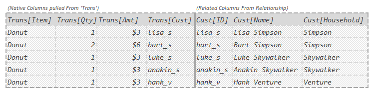
So ideally some version of the above is the image you should see in your head when your eyes glance over “Trans” in our Measure:

Households Sold To =
COUNTROWS(
    GROUPBY( Trans, Cust[Household] )
)

For arguments 2+ of GROUPBY we could have typed in any combination of column names from the above Temp Table and GROUPBY would bring back their unique combinations. We kept it simple though. We only type in 1 column name: “Cust[Household]”. In other words:

“Hey GROUPBY, you see this Temp Table? I want you give me just the unique values of the last column in it which is called “Cust[Household]”.

So GROUPBY looks at the Temp Table we handed it:

It then finds the column called “Cust[Household]” at the end, and produces a new Temp Table with just that one column’s unique values. (The duplicate values for “Simpson” and “Skywalker” get dropped):

Hey look, it’s a Temp Table of all the households we sold donuts to. If we could count how many rows were in that Temp Table, we’d have our answer.

Which is in fact what our code does next. That Temp Table gets sent to COUNTROWS, which has the rather boring but important job of looking at that Temp Table and saying “3”.

Yep, 3, that’s our final answer.

Here’s the whole thing zoomed out:

The reference to “Trans” is an Auto Snapshot of the “Trans” Model Table producing a Temp Table with 5 rows and 7 columns (4 Native columns plus 3 Related columns).

We give that Temp Table to GROUPBY and tell it to keep all the unique values of the “Cust[Household]” column. GROUPBY spits out a Temp Table with just those values in it.

This last Temp Table is then given to COUNTROWS which says “That Temp Table has 3 rows in it”.

Easy as that.

Is this realistic though? Absolutely. I use variations of this simple pattern probably a couple times a week.

Importance of Visualization

So this series isn’t about GROUPBY, it’s about the Auto Snapshot and why it’s helpful to be able to visualize it properly.

With that in mind let’s rewind and imagine you are trying to write our Measure from scratch.

Somebody has told you that you need to design a Measure that calculates how many households we have sold to (and it needs to respond to slicers).

OK.

Step 1: You create a Measure and give it a name:

Step 2: ???

Now what? You know you are supposed to calculate the total number of households sold to, but how? This isn’t a simple SUM, that won’t work. Normally you’d use DISTINCTCOUNT for something like this, but when you try that, it ignores the slicer set for Donut which needs to work.

If instead of starting by trying to figure out which function you need, you simply think:

“This is relates to transactions, what would the Auto Snapshot of “Trans” give me?”

If you can then envision some version of this in your head:

You will probably immediately look at that last column and think:

“If I can just get all the unique values of that last column and count them, I’ll have my answer.”

And you would be right. You still have to go find the function that does that “getting the unique values” bit. A tiny bit of research later you’ll find that the GROUPBY and SUMMARIZE functions both can do that (for this demo you could use either and you would use them the exact same way).

Just like that, your measure is written in less than a minute:

Households Sold To =
COUNTROWS(
    GROUPBY( Trans, Cust[Household] )
)

Being able to see the result of the Auto Snapshot in your head will make writing lots of DAX much much faster and easier.

By contrast. Imagine when you start writing the Measure you head to the Data Viewer in Power BI and just stare at this table:

You’ll probably get frustrated quickly and assume the problem is a lot harder to solve than it is.

If you start by seeing the Auto Snapshot in your head, a huge number of problems, just like this, go from vexing to almost obvious.

OK. Cool story Brian.

One small problem.

How in the world do you get good at seeing the Auto Snapshot in your head?

This took me years to get good at; and even then, the images I see in my head are not nearly as high fidelity as the ones I’m showing you. That said, you don’t have to get to my level to derive value from this; a little goes a long way.

Getting good at this is indeed a skill, but it’s a skill worth doing. Like I said at the start Table Vision is the most important skill in DAX. If you can see the tables in your head, even poorly, the language starts to get easy. Until you do, the language is impenetrable. The sooner you start climbing, the sooner you get up the mountain.

In the next post I’ll try and help you see the Auto Snapshot as I see it in my head. That will help you wake up these muscles so you can start making your way up the mountain.

-BG