
In the last post we finished our introduction to Evaluation Context. The short story is that every formula and sub-formula in DAX runs with two lists in place.
The first is a list of all the values in the current row; this list is called “Row Context”. The second is a list of all the filters currently active; this list is called “Filter Context”. Together these two lists make up what is called the “Evaluation Context” of a sub-formula.
Here’s a picture of an example Evaluation Context to make things more concrete:
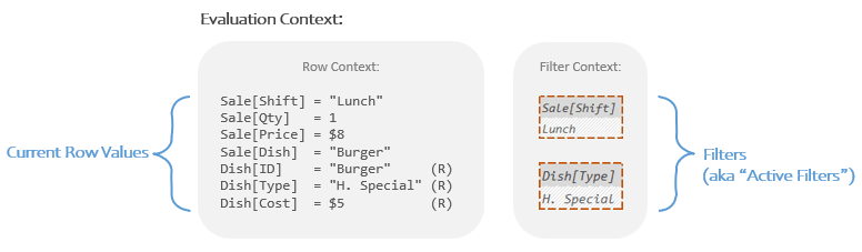
The job of the CALCULATE function is to build a new Evaluation Context where changes have been made to the Filter Context, and then run a sub-formula in that new Evaluation Context. We call this sub-formula a “New Filters Formula” because it’s the formula that runs with the new list of filters in place.
In the last post, because I was focusing on just the concept of Evaluation Contexts, I showed you the simpler example of CALCULATE where you remove a filter rather than add one. In this post I will show you how to add one. If the filter you want to add is complicated, this can be, well, complicated. However if the filter you want to add is simple (“I want to add a filter for dinner”) then this is quite easy.
Here, let me show you.
The Concept
All you have to do if you want to use CALCULATE to add a filter to the Filter Context is give it a Temp Table. That’s it. Really.
Let’s look at what you are supposed to type into CALCULATE to make this happen:
CALCULATE(
    <This Is Where You Write Your New Filters Formula>,
    <This Is Where You Write Instructions For A Temp Table>
)
Argument 1 is something we’ve covered quite a bit, that’s where you type in your New Filters Formula.
Argument 2 is where you type in your Filter Modification; which will look a little different depending on whether you want to add or remove a filter. In the last post we wanted to remove a filter so we used the REMOVEFILTERS function. To add a filter you don’t have to use some specialty function with a name like ADDFILTERS (no such function exists); instead you simply type out any set of instructions for building a Temp Table. Since all filters in DAX are Temp Tables, if you type out instructions for building a Temp Table, CALCULATE will assume that what you want is for that Temp Table to get built and then added as a filter in the Filter Context. We call this “giving” or “passing” a Temp Table to CALCULATE.
Wait…
How do you write instructions for building a Temp Table?
That’s where things get more complex (but just a little).
For simple filters there are about 3 ways to do it.
I’m *not* going to show you the most common method people use; it looks easiest, but understanding how it works is very hard. I’m instead going to show you the method that strikes a great balance of being relatively easy to understand, but not relying on a lot of smoke and mirrors.
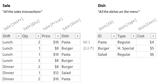
Our Model
This is the same Data Model as always:
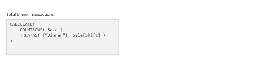
Let’s say we want a Measure called “Total Dinner Transactions”; which should count the number of rows, but always only looking at the Dinner Shift.
Here’s the finished version. To keep things simple I’m leaving the both slicers empty.

(Did you catch the part where I’m leaving both the slicers empty? That’s different than before.)
So what is this miraculous Measure?
Total Dinner Transactions =
CALCULATE(
    COUNTROWS( Sale ),
    TREATAS( {"Dinner"}, Sale[Shift] )
)
(I’ve highlighted argument 2, which are the instructions for creating our Temp Table.)
If your eyes just went real wide; stop and take a breath. This isn’t supposed to make sense yet and it’s much easier than it looks.
To start understanding it, we have to take a brief diversion into both Quick Tables and the TREATAS function.
Quick Tables: Temp Tables the Easy Way
So in DAX if you want to build a Temp Table quickly without a lot of fuss you can just use the little curly braces. I call these Quick Tables, though the more official name is the “Table Constructor”. The name isn’t super important here. What’s important is you can build simple Temp Tables quickly using curly braces.
So let’s say I want to quickly build a single column Temp Table with the numbers 10, 25, 200 and 499 in it. I could write this:
{ 10, 25, 200, 499 }
That builds a Temp Table that looks like this:

That Temp Table can be given to any function that uses Temp Tables, including functions like COUNTROWS or SUMX or CALCULATE. It will just work.
Where did the column name of “[Value]” come in? It’s just the name you get when you create a Quick Table with the curly braces. The whole idea is that you want to build a Temp Table quickly without a lot of fuss, and the name of the column usually isn’t important; so DAX just gives it these names by default.
Can you build a Quick Table with text instead of numbers? Yep.
So:
{ "Canada", "United States", "Mexico" }
Produces this Temp Table:
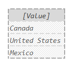
(Notice that in your code, text values need to be in quotation marks but numbers do not; just like Excel)
Can I produce a Quick Table with more than one column? Sure! You just add pairs of regular parenthesis inside the curly braces to define the rows.
So this:
{ ("Coffee", 10), ("Tea", 20 ) }
Creates this Temp Table:
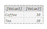
The stuff in the first set of parenthesis is row 1, the stuff in the second set of parenthesis is row 2. Notice also that with the 2+ column version the column names switch from “Value” to “Value1”, “Value2”.
Also, you’d usually rewrite the above with some spacing and line breaks to make it easier to read. Something like this:
{
    ( "Coffee", 10 ),
    ( "Tea",    20 )
}
You don’t have to, the computer won’t care if you write it with spaces and line indentation or not. That said, it’s good to both spaces and line indentation to make your code easier to read for both your coworkers and also future you.
Here’s one more big example:
{
    ( "Alaska",     "Anchorage",     733391 ),
    ( "Washington", "Olympia",      7705281 ),
    ( "Idaho",      "Boise",        1839106 ),
    ( "Oregon",     "Salem",        4237256 ),
    ( "California", "Sacramento",  39538223 ),
    ( "Nevada",     "Carson City",  3104614 ),
    ( "Hawaii",     "Honolulu",     1455271 )
}
Creates this Temp Table:

(Not that it matters, but those are several Western U.S. states, along with their state capitals and state populations.)
Notice we have 3 columns in this one and the third column is just called “[Value3]”. While it’s definitely possible to create Quick Tables that are really long and really wide, most of the time they will have only 1 column and just a handful of rows.
Are Quick Tables a different kind of table than a Temp Table? Nope.
Quick Tables are just a specific *way* of creating a Temp Table. Whenever you are using the curly braces in DAX, you will produce a Temp Table. When you produce a Temp Table this way, it can be called a Quick Table.
These have several uses, but the most common by far is creating simple filters. Let me show you how that works.
TREATAS Yourself
OK, so if we want to create a filter for Dinner we first need a Temp Table with the value of Dinner in it.
You probably guessed I can just do this:
{ "Dinner" }
And it gives us this Temp Table:
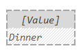
The problem is that we want our filter to do filtering on the “Sale[Shift]” column. Since the column name for the Temp Table above is “[Value]” it won’t do that. Essentially have to rename that column from “[Value]” to “Sale[Shift]” if we want it to work properly.
That’s where the TREATAS function comes in. While I’m simplifying a little, basically, you give it a Temp Table (argument 1), and then give it what you’d like the new column names of that Temp Table to be (arguments 2+).
So:
TREATAS( { "Dinner" }, Sale[Shift] )
Basically takes this Temp Table:

And makes a copy of it with the column renamed to “Sale[Shift]” like this:
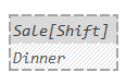
There we go, that’s the exact Temp Table we want to add as a filter. It’s got the value we want and the correct column name so that when used in Auto Filtering it will filter on the “Sale[Shift]” column to keep just the “Dinner” rows.
So again, we use the Quick Table to create the initial Temp Table, then use TREATAS to rename the column so it will work properly as a filter. I’ll want to circle back to TREATAS in another post to talk about some important subtleties I’m skipping over, but for the most basic use, you can just think of TREATAS as “that function that renames columns so they can be used as filters“. That’s good enough for an introductory post.
OK, back to CALCULATE!
All Together Now
OK, now we want to try and visualize how this Measure works.
First, let’s imagine our Measure floating in its own little box:
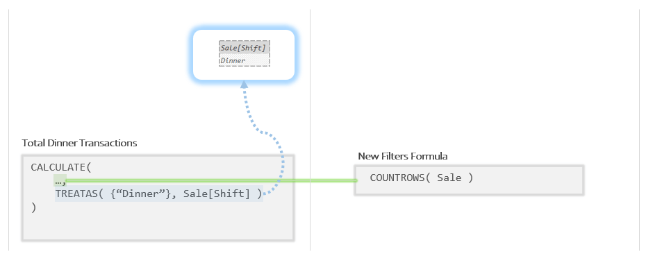
And now let’s decompose it by breaking the sub-formula out into it’s own little box:

Now we can see both the parent formula and the sub-formula broken out. The idea is that CALCULATE is going to build a new Evaluation Context for the New Filters Formula to run in.
OK, before I draw in both the initial and the new Evaluation Contexts, I want to add in the Temp Table that the TREATAS functions is giving to CALCULATE:
Now I’m going to add the Evaluation Contexts for both sides. Keep in mind that in this example, the user hasn’t clicked on any slicers, so the first Evaluation Context will be empty:
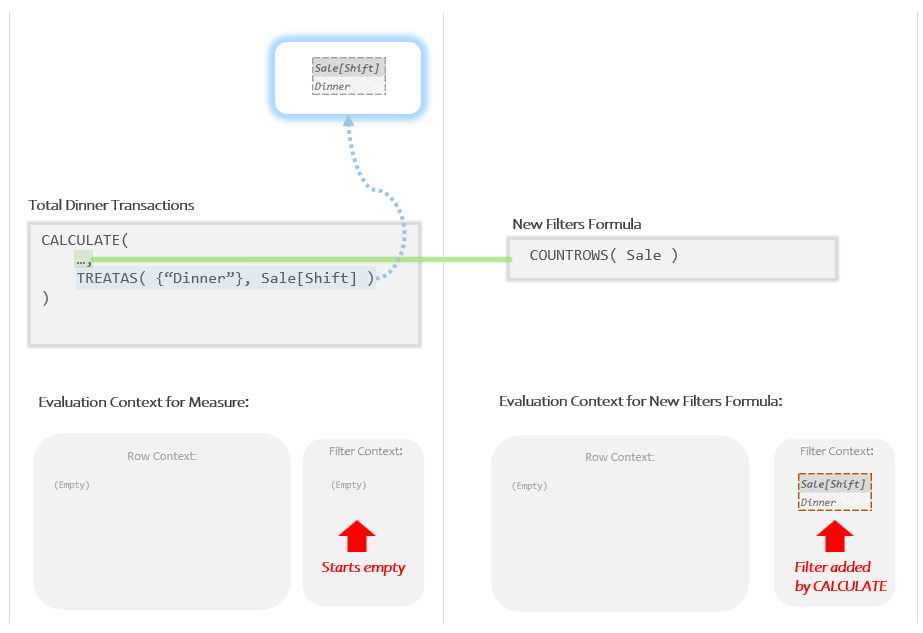
So the Initial Evaluation context is empty (the user hasn’t clicked on a slicer). CALCULATE made a copy of this Evaluation Context and added the Temp Table we handed it as a filter.
It’s that new Evaluation Context that the New Filters Formula runs within. It’s going to take the Auto Snapshot of “Sale” and give it to COUNTROWS. Let’s draw in what the Auto Snapshot produces:
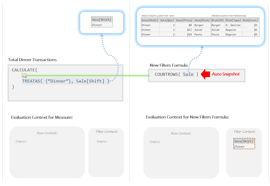
The Auto Snapshot produces just the 3 Dinner rows as a Temp Table. During the Auto Filtering phase of the Auto Snapshot the “Dinner” filter got applied knocking the initial 7 rows down to 3.
When COUNTROWS is given that Temp Table, it returns 3 which is the answer we see in Power BI.
Just like last time I want to draw a separate illustration just for the Auto Snapshot occurring in the new Filter Context. I’m not going to show you this full process every time, but I want to make clear where the Filter Context got used:
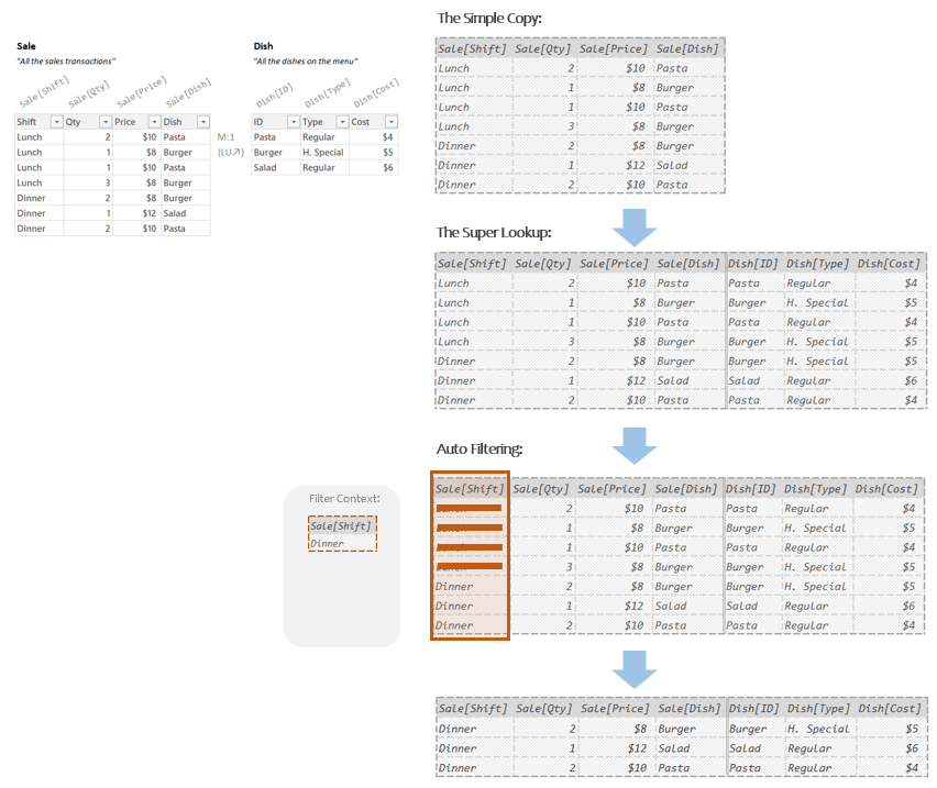
Notice that in the Auto Filtering step, it is that new Filter Context that DAX uses to determine which filters to apply. The Measure’s initial Filter Context had zero filters (no slicers were clicked on) but CALCULATE built the new Filter Context for the New Filters Formula with the added “Dinner” filter. Every time Auto Filtering happens in any New Filters Formula, it uses the new Filter Context to know what filters to apply.
So that last Temp Table at the bottom is what COUNTROWS gets and so it returns the number 3.
That is our final answer:

Winding Down
For simple filters like our example this is very easy. More complex filters will require more sophisticated techniques, but we have to really understand the simple stuff first. In the next post I’m going to just show you several more examples of this just to help cement the idea in your head.
After that, I can finally show you one more very important thing that you can do with CALCULATE called “Context Transition”. It sounds scarier than it is; but is very important to master either way. That’s coming soon.
Till next time!
-BG
Post Script: The Good, The Bad, and The Ugly
If you’ll remember at the beginning I said there were 3 ways to set a simple filter using CALCULATE, let me show you examples of all 3:
Total Dinner Transactions V1 =
CALCULATE(
    COUNTROWS( Sale ),
    TREATAS( {"Dinner"}, Sale[Shift] )
)
Total Dinner Transactions V2 =
CALCULATE(
    COUNTROWS( Sale ),
    Sale[Shift] = "Dinner"
)
Total Dinner Transactions V3 =
CALCULATE(
    COUNTROWS( Sale ),
    FILTER( ALL( Sale[Shift] ), Sale[Shift] = "Dinner" )
)
All three version above produce the exact same result. I’ll pull out the highlighted bits from all three so we can look at them in isolation:
Version 1:
TREATAS( {“Dinner”}, Sale[Shift] )
Version 2:
Sale[Shift] = “Dinner”
Version 3:
FILTER( ALL( Sale[Shift] ), Sale[Shift] = “Dinner” )
Most folks look at the above options and love version 2 and hate the others.
This is understandable. Version 2 is usually what most books and classes (including a lot of my own) tell you to do when starting out. There’s a problem with version 2 though: version 2 is actually a shortcut way of writing version 3. Which is to say, when you write version 2 into CALCULATE, the first thing that DAX always does is rewrite it as version 3. If you’ve been using version 2 for years, DAX has been rewriting it for you as version 3 this whole time.
You can start to see this if you line them up correctly:
Version 2: Sale[Shift] = “Dinner”
Version 3: FILTER( ALL( Sale[Shift] ), Sale[Shift] = “Dinner” )
Version 2 is just the little bit that appears near the end version 3. Specifically, it is just the Per Row Formula of FILTER in that version. OK, fine; but why does rewrite it?
Since in DAX all filters are Temp Tables, CALCULATE needs to know *how* to build the Temp Table you want it to add as a filter. When DAX looks at version 3 it sees all the steps needed to create a Temp Table written out explicitly. When it looks at version 2 it sees just a partial set of instructions that only makes sense if DAX rewrites it as version 3.
Said otherwise, version 2 only counts as “instructions for building a Temp Table” if DAX fills in a bunch of steps you left out. As far as DAX is concerned it is like a sentence fragment; that is to say, a sentence that is missing some important pieces.
Version 2 is the equivalent of walking up to someone in a foreign country and saying “Please museum?” in the local language. The person can guess that you are trying to say something like “Please, could you point me in the direction of the museum?”, but to do so they have rewrite your clumsy sentence in their head. You are not actually asking them where the museum is, but they can figure out that that’s what you want and will probably help you out.
If you’re visiting a country for a couple days, wandering around saying thinks like “Please museum?”, “Please train station?”, or “Please bathroom?” is probably OK (if you are being very polite about it) however you should not delude yourself into thinking you understand the local language. If you want to live there or do business there, you really need to learn how to speak in complete sentences.
For casual DAX authors, version 2 is fine; DAX can take the clumsy partial instructions and fill in the gaps. If you want to get really good at DAX, you need to be able to write it in a way where DAX isn’t constantly filling in the gaps for you. That means you should avoid version 2 when starting out.
OK, so version 2 is out. So why version 1 rather than version 3?
Let me show them to you side by side:
Version 1: TREATAS( { “Dinner” }, Sale[Shift] )
Version 3: FILTER( ALL( Sale[Shift] ), Sale[Shift] = “Dinner” )
The short answer is that version 1 is preferable because it is simpler to understand. You create a Quick Table with the curly braces, then use TREATAS to rename its column.
Version 3 involves a Snapshot, an Iterator, and a Per Row Formula. This is by no means impossible to understand but it is harder. When we’re focusing on trying to learn CALCULATE, the simplicity of version 1 lets you focus on learning how CALCULATE works so you’re not trying to understand two ideas at once.
OK, with all that I’m going to give you some mnemonic names to help remember the different versions:
“The Good”
TREATAS( { “Dinner” }, Sale[Shift] )
“The Bad”
Sale[Shift] = “Dinner”
“The Ugly”
FILTER( ALL( Sale[Shift] ), Sale[Shift] = “Dinner” )
“The Good” is good because it is explicit about what it’s doing and is fairly easy to read.
“The Bad” is bad because it doesn’t communicate what it’s doing.
“The Ugly” is ugly because it’s the hardest to read.
DO NOT read too much into these names. I picked them because they are very useful for understanding the *tradeoffs* between the three for people trying to *understand” DAX and are easy to remember; but in term of *performance* all 3 work equally well. Using “The Good” doesn’t mean you are a better DAX author; it’s just the most helpful in understanding what DAX is doing for a new author. I write “The Bad” version all the time, because I know how to look at it and rewrite it in my head so I can see what it’s doing mechanically. I am not asking you to stop using “The Bad” version; but when you use it, I would suggest you pause and see if you can both rewrite it into “The Ugly” version your head (just like DAX has to do), and more importantly see in your head how it is going about creating the Temp Table you want.
DAX is a language that manipulates tables in various ways in order to produce numbers that are useful to people. Code that makes clear how you are manipulating the tables will help you understand what’s happening and what might be broken. Code that only conveys what you want the end results to look like will by prevent you from seeing what DAX is *doing* to come up with a number. If you can’t see what it’s doing, you will never be able to spot what’s broken or what can optimized. Writing “table-centric” code is your friend. Hence my bias towards “versions 1 and “The Good” and “The Ugly” for new authors.
(As a last ask, if you are taking a class and they use “The Bad” version, please don’t raise your hand and ask why they are teaching things “The Bad” way. “The Bad” way exists because learning things “The Good” or even “The Ugly” way is too difficult for most new students to understand and requires an enormous amount of setup for what won’t feel like a big difference for students.)
